LWE to RLWE Conversion

This article builds on the LWE to LWE Key Switching. Read it first before proceeding with this one.

Here, we introduce the concept of converting LWE to RLWE ciphertexts which is the second contribution of the CDKS paper.

It is helpful to convert between the different encryption schemes since:

• LWE is simpler and works well for lightweight encryption.
• RLWE is more efficient for complex homomorphic computations. RLWE can leverage NTT-accelerated multiplication to achieve faster operations

In the previous article, we introduced polynomial embedding, which allows us to convert LWE into a valid RLWE ciphertext. As noted, the embedding produces a polynomial with correct constant term but garbage elsewhere. To make this a valid RLWE encryption of the scalar message $\mu$, we must zero out the non-constant coefficients.

The mathematical tool that accomplishes this is called the Field Trace.

Field Trace

Field trace $\text{Tr}_{K/\mathbb{Q}}$ is a mathematical "filter" that zeroes out all non-constant terms while retaining the constant. This is exactly what we need to cancel out the garbage in the embedded RLWE ciphertext.

Here, $\mathbb{Q}$ denotes the rational numbers and $K = \mathbb{Q}[X]/(X^N + 1)$ is the cyclotomic field — the number field in which our RLWE polynomials live. The details are not important for intuitive understanding but can be found in the original paper.

But how does the field trace achieve this filtering effect? The answer lies in the concept of Symmetrization.

Symmetrization

Symmetrization relies on two fundamental concepts:

• Invariance (things that stay the same)
• Cancellation (things that balance out)

In the context of a polynomial:

• The constant term (a simple integer) looks the same from every view. It is invariant.
• The variable terms ($X, X^2, \dots$) change with every view.

Mathematically, these different "views" come from the Galois group — automorphisms that rotate the root of unity $\zeta$ (represented by $X$) to other valid roots. But the intuition is simpler:

Think of each automorphism as looking at the polynomial from a different, symmetric angle.

• The Constant Term ($\mu_0$): This is a simple integer. It is invariant. No matter how you "rotate" the coordinate system ($X$), an integer like $\mu_0$ remains $\mu_0$.
• The Variable Terms ($\mu_i X^i$): These depend on $X$. When you apply an automorphism, these terms rotate to point in different directions in the complex plane.

When you sum them all up, the invariant parts (constants) add up constructively, while the variable parts cancel each other out (destructive interference).

The Field Trace is the sum of all these different views. When you perform this summation, two distinct physical-like phenomena occur:

1. Constructive Interference (The Message) Since the constant term $\mu_0$ is invariant, it looks exactly the same in every view.

• If you have $N$ views, and in every view the value is $\mu_0$, the sum is simply:

$\mu_0 + \mu_0 + \dots + \mu_0 = N \cdot \mu_0$

The signal reinforces itself.

2. Destructive Interference (The Garbage) The variable terms are roots of unity. A key property of these roots is that they are perfectly distributed around the unit circle (see visuals below).

• For every view where a term $X^i$ is positive, there is a symmetric view where it is negative.
• For every vector pointing "up," there is one pointing "down."
• When you sum all these symmetric vectors together, they perfectly balance each other out to zero.

$\sum \text{All Rotations of } X^i = 0$

Visual Intuition

Let's now visualize how Galois automorphisms rotate roots of unity, causing variable terms to cancel.

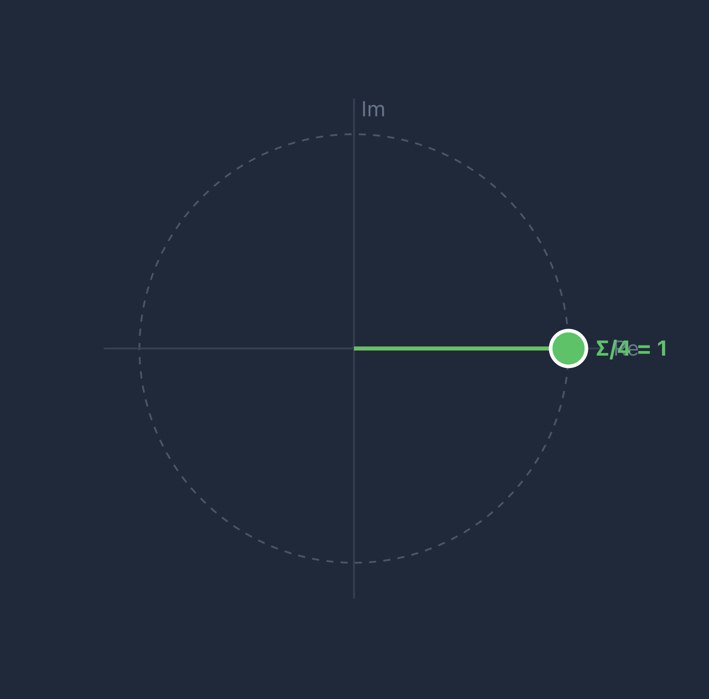
For a term $X^i$ with $N=4$, the trace is:

$\text{Tr}(X^i) = \sum_{k=0}^{N-1} \zeta^{ki}$

For the constant term ($i = 0$), every $\zeta^{k \cdot 0} = 1$. All $N$ vectors point to $(1, 0)$, giving a sum of $N$. This is the message that survives.

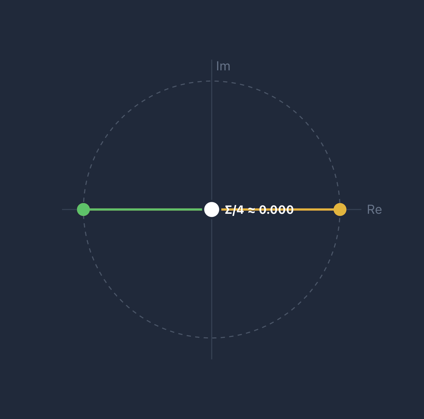
When $N$ does not divide $i$, the roots are evenly distributed around the unit circle, so their sum is $0$ — this is the destructive interference that cancels the garbage. For example, with $X^2$ and $N=4$, each root $\zeta^k$ gives $(\zeta^k)^2 = \zeta^{2k}$. These 4 points are evenly distributed around the circle, so their sum = 0.

To summarize, the Field Trace essentially asks: "What part of this polynomial is true from all perspectives?"

• The variable terms are only "true" from specific angles, so they cancel out when you average over all angles.
• The constant term is true from all angles, so it survives and amplifies.

This effectively projects the complex, multi-dimensional polynomial down to its single, stable scalar component (the LWE message).

Trace Algorithm

Computing the trace directly by summing $N$ automorphisms (for each term $X^i$) would require $O(N^2 \log N)$. Instead, we use a recursive approach that requires only $\log N$ steps.

Definitions

Before running the algorithm, let's define the "ingredients":

• $N$ (Dimension): The size of the polynomial ring (e.g., 4096 or 8192). It represents the total number of coefficients in our polynomial.
• $q$ (Modulus): The large integer that defines the "clock" for our arithmetic (we calculate modulo $q$).
• $ct = (b, a)$ (Ciphertext): A pair of polynomials representing encrypted data.
• Embedded LWE: A specific ciphertext where the message is hidden in the constant term (coefficient of $X^0$), and all other $N-1$ coefficients contain garbage that we need to zero out.
• $\tau_d$ (Automorphism/Rotation): The automorphism $\tau_d: X \mapsto X^d$, which permutes the coefficients of the polynomial. Think of it as "spinning" the polynomial by index $d$.
• $d_k$ (Rotation Index): An integer that tells the Automorphism function how much to spin the polynomial at step $k$.
• $\ell$ (Decomposition Dimension): The number of digits in the gadget decomposition from key-switching, typically $\ell = \lceil \log_B q \rceil$ where $B$ is the gadget base.
• $\text{EvalAuto}(ct, d_k)$: Applies the automorphism $\tau_{d_k}: X \mapsto X^{d_k}$ to the ciphertext. Internally, this requires key-switching (see previous article) to re-encrypt under the original key after rotating.

Intuition: Divide and Conquer

To understand why the trace algorithm is fast, compare the Naive Approach vs. the Recursive Approach.

The Goal: We have 1 good term (Constant) and $N-1$ bad terms (Garbage). We want to sum different "views" (rotations) of the ciphertext so that the bad terms cancel out to zero.

The Naive Approach (Linear)

Imagine trying to zero out the garbage by targeting every single term individually. You would need $N$ separate rotations to kill $N$ different variable terms.

• Cost: $N$ steps. If $N=4096$, that is 4096 operations.
• Complexity: $O(N^2 \log N)$.

The Recursive Approach (Logarithmic)

Instead of targeting terms one by one, we target half of the remaining terms at every step.

1. Perform a rotation that turns all odd powers ($X, X^3, X^5...$) negative. When you add this to the original, 50% of the garbage vanishes instantly.
2. Perform a rotation that turns half of the remaining even powers ($X^2, X^6...$) negative. Add it. Now 75% of the garbage is gone.
3. Repeat.

• Cost: You only need to halve the pile $\log N$ times to reach 1. If $N=4096$, $\log_2(4096) = 12$. You finish in 12 steps instead of 4096.
• Complexity: $O(N \log N)$.

The Algorithm

Input: $ct_0 = (b, a)$ (Embedded LWE)

Loop: For $k = 1$ to $\log N$:

• $d_k = 2^{\log N - k + 1} + 1$
• $ct_k = ct_{k-1} + \text{EvalAuto}(ct_{k-1}, d_k)$

Why these rotation indices?

The index $d_k = 2^{\log N - k + 1} + 1$ is engineered so that half the surviving coefficients at iteration $k$ land in positions where $X^N = -1$ kicks in, flipping their signs.

Adding $ct_{k-1} + \tau_{d_k}(ct_{k-1})$ cancels these flipped terms.

The "+1" ensures $d_k$ is odd — a requirement for valid automorphisms in the cyclotomic ring.

Output: $ct_{\log N}$

Complexity:

• This approach requires evaluating $\log N$ automorphisms
• Each automorphism evaluation costs $O(\ell N \log N)$ due to key-switching (with $\ell$ gadget digits) and NTT operations
• Total Operations: $\log N \times O(\ell N \log N) = O(\ell N \log^2 N)$

Summary

The LWE-to-RLWE conversion uses polynomial embedding followed by the Field Trace operation to project an embedded LWE ciphertext onto a clean RLWE encryption of the original scalar message. The recursive trace algorithm makes this conversion practical, requiring only $O(\log N)$ automorphism evaluations instead of $O(N)$.